Description of the method

The following is only a description of the parts of the RECOVERY algorithm relating to the special features of the $\mu SR$ experiments. The detailed description of the algorithm and its applications can be found in papers [7] and [8].

In $\mu SR$ experiments, scintillating counters detect the muon's decay positron, the direction of which is correlated with the muon spin direction at the time of its decay. The number of decay positron is histogrammed as a function of the time taken to decay

 

$$N(t) = N_0 [1 \pm A_{Mu} \cdot P(t)]e^{-t/t_{\mu}} + B,$$ (8)

where $t_{\mu}=2.197 \cdot 10^{-6}~s$ is the muon life time, N₀ is proportional to the intensity of muon beam, A_Mu is the asymmetry coefficient, and B is the random background level. It is worth noting that the sign before the asymmetry coefficient A_Mu may be plus or minus for two opposing scintillating counters which are along (+) or opposite (-) of the initial muon spin direction [2],[6].

The polarization function P(t) in Eq.(8) can only be uniquely determined from the histogram N(t) if all parameters N₀, B and A_Mu are known. We chose to pre-determine the parameters N₀, B and A_Mu using the crude standard $\mu SR$ analysis method (using Eq.(9) below) and then use those values to extract the generalized P(t) from the experimental N(t).

For the first step of determining N₀, B and A_Mu, we use the fact that in temperature range 0.5 - 1.5 K the muonium formation time t₀ is less than the total histogram duration $t_1 \approx 10~\mu s$ and for $t \geq t_{0}$, when all atoms of muonium have been formed, the equation for histogram can be written as

 

$$N_1(t) = [A+C \cos(\omega_{Mu}t) + D \sin(\omega_{Mu}t)]e^{-t/t_{\mu}} + B.$$ (9)

Now we can easy find all of four parameters A,B,C, and D by minimization of the value

$$\chi^2 = \displaystyle\sum_{t_i>t_{0}}\frac{[N(t_i)-N_1(t_i)]^2}{N(t_i)} \,.$$ (10)

It has taken into account that the experimental data N(t) have a Poissonian distribution. This procedure can also be used to determine the value of the magnetic field projection on the axis of muon spin precession.

The system equation originating from the minimization of Eq.(10) has a symmetric and positive-definite matrix. We solve this system by the Cholesky decomposition method (square root of matrix) with the subroutines CHOLSL and CHOLDC from the 2nd edition of the "Numerical Recipes" book by W.H.Press et al [10]. These programs were modified for double precision ( ${real\ast8}$) accuracy. The use of the Cholesky decomposition method for a symmetric and positive-definite matrix provides more stable results than the Gaussian elimination method which does not use the symmetry properties of the matrix.

With values for the parameters A,B,C and D we compute N₀ and asymmetry coefficient A_Mu using the formulas

$$N_0=A \displaystyle \exp(t_{0}/t_{\mu}),\;\; A_{Mu}=\displaystyle \frac{\sqrt{C^2+D^2}}{A}.$$ (11)

We now know all parameters in Eq.(8) and we can now solve this equation for the polarization function

$$P_2(t)=\frac{1}{A_{Mu}} \left[ 1-\frac{N(t)-B}{N_0} e^{t/t_{\mu}} \right] .$$ (12)

The polarization function P₂(t) starts from the initial value

$$P_2(0) \simeq 2$$

and degrades rapidly into the regime of oscillating between +1 and -1. This reflects the fact that one half of polarization only remains after the formation of muonium atoms [2].

Traditionally another normalization is used

P(0)=1,

and in this paper we compute the polarization function as

$$P(t)=\frac{P_2(t)}{\hat{P}_2(0)}.$$ (13)

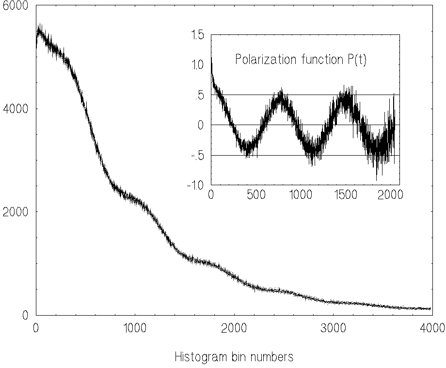
Here $\hat{P}_2(0)$ is the estimate of the function P₂(t) for time t=0 from its first 16 initial values obtained by using the optimal filtering program [11]. After an initial time, the function P(t) oscillates between +1/2 and -1/2. The original histogram N(t) and polarization function P(t) calculated using Eq.(13) are shown in Fig.1 for helium at a temperature of 0.7K.

Fig.1. Input histogram and polarization function P(t) for the first 2048 data points (in insert). Temperature T=0.7K, histogram bin number N=3983, one bin time $\Delta t=2.5$ ns.

It is obvious in Fig.1 that the noise level in function P(t) increases with t. This level can be easy seen from the the fact that N(t) has a Poissonian distribution which results in

var[N(t)]=N(t).

If we approximate

$$N(t) \approx N_0 e^{-t/t_{\mu}},$$

then from Eqs. (12) and (13) we obtain

$$var[P(t)] \approx \displaystyle \frac{1}{A_{Mu}^2N(t) {\hat{P}_2}^2(0)}$$ (14)

This formula for estimation of noise level in polarization function P(t) is used in the algorithm presented in this paper.

After these appropriate preliminary calculations let us go to the main problem of this paper: how to determine the muonium formation rate function n(t) in a model independent way, that is without assuming any particular theoretical form with fit parameters for the polarization function P(t).

Eq.(7) can be rewritten as

$$P_1(t)= \int \limits_{0}^{t} n(t') \left[\frac{\cos\omega_{Mu}(t-t')}{2}-1\right] dt',$$ (15)

where

 

P₁(t)=P(t)-1. (16)

Eq.(15) is the Volterra convolution integral equation of the first kind with the kernel

$$K(t-t')= \frac{\cos \omega_{Mu}(t-t')}{2} -1$$ (17)

which is used to recover the nonnegative function n(t) from the input data P₁(t).

To solve this integral equation we use the program Dconv2 from the program package RECOVERY. The program Dconv2 was originally designed for the solution of the Fredholm integral equation with fixed integration limits

$$P_1(t)= \int \limits_{0}^{T} n(t')K_1(t-t')dt'.$$ (18)

To use the program Dconv2 for the Volterra integral equation, we modified the kernel as follows:

$$K_1(t-t') = \left\{ \begin{array}{ll} K(t-t'), &t' \leq t, \\ 0, &t' >t. \end{array}\right.$$ (19)

The data arrays in the upgraded program have been increased to handle 2048 input points for use with $\mu SR$ histograms.

The program package RECOVERY, which is based on the maximum likelihood method (MLM), was chosen because this method attains the maximum possible resolution enhancement for a given signal to noise ratio in the input experimental data [7]. According to the MLM, the likelihood function

$$L = {\cal P}(F\vert G_0),$$ (20)

should be first defined, where ${\cal P}(F\vert G_0)$ is the conditional probability of observing a set of experimental data points

$$\{F_i\},\;\;i=1,2,...,n,$$

which coincides with the real data set, providing that the solution is G₀. In our case G₀ is the muonium formation rate n(t).

Consider the set of unknown values of the function G₀(y_j), j=1,2,...,m as a vector in an m-dimensional space of solutions. Each point in this space corresponds to one possible solution, and the next step is to search for the likelihood function maximum

$$max {\cal P}(F\vert G_0),$$

on a set of solutions limited by some necessary restrictions. For many problems, including the muonium formation rate problem, an important condition is that the solution is not negative.

An explicit form of the likelihood function for the case of polynomial statistics is given in review paper [12]. Poissonian statistics are a special case of polynomial statistics. If the data are described by Gaussian statistics, then the logarithmic likelihood function is the square of deviation between the experimental data $\{F\}$ and their approximation $\{\hat{F}_0\}$, i.e.

$$\log L=const-\displaystyle\frac{1}{2}\parallel F-\hat{F}_0\parallel.$$

Here the two vertical lines denote the square norm and

$$\hat{F}_0=K\hat{G_0}$$

is the integral transform (15) or (18) of the trial solution $\hat{G_0}$.

The search for the likelihood function maximum is performed iteratively by the steepest ascent method which is a sign-inverted variant of steepest descent method. All explicit formulae of iterative algorithms for both polynomial and Gaussian input data statistics can be found in reference [8] and a full listing of the RECOVERY code in Fortran 77 is available from the CPC Program Library providing that person requesting the program sign the standard CPC non-profit use licence. The more sophisticated conjugate gradient method is used in this paper for maximization of the likelihood function.

The number of detected positron in one time bin in our measurements was about 10³ - 10⁴ and it is well known that for such large numbers of events Poissonian statistics are reduced to Gaussian. It follows from the Eq.(14) that the variance of input data P(t) is inversely proportional to the histogram values N(t) and the main subroutine MLG8 should be used together with the program Dconv2. This subroutine is designed for input data having the Gaussian statistics with non-constant variance (see part 2 of paper [8]).

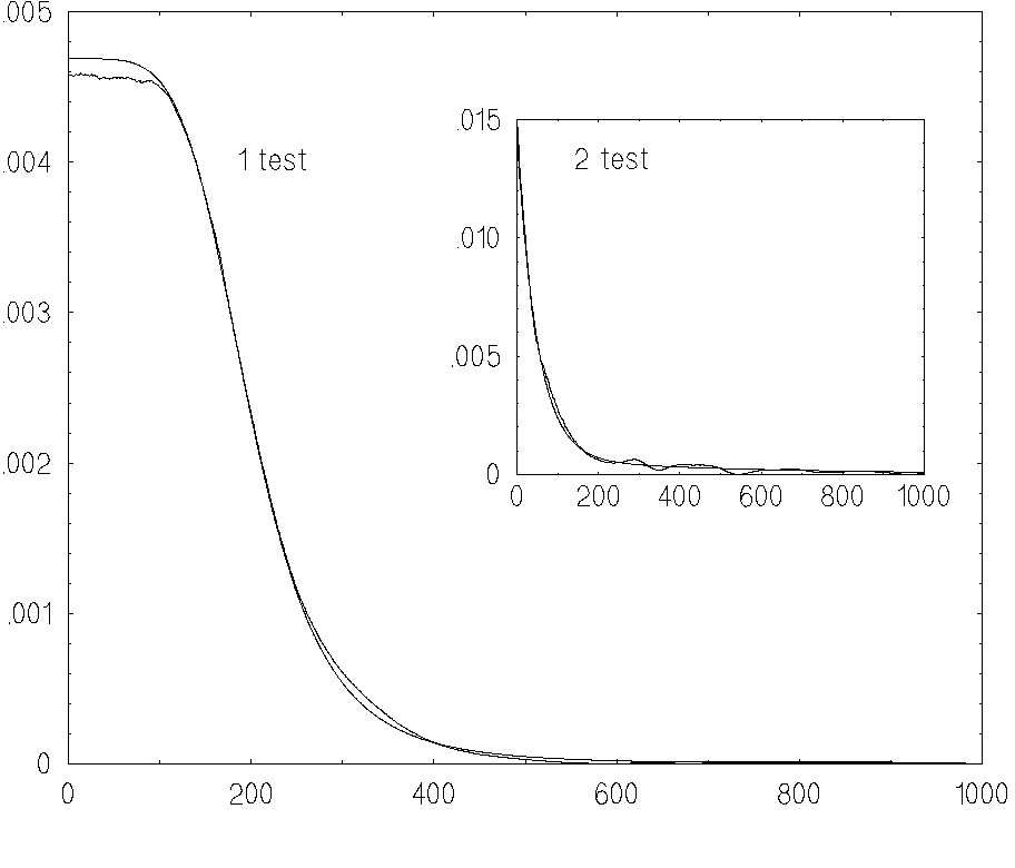
To demonstrate that our RECOVERY procedure is unbiased with respect to the analytical form of formation rate function n(t) we choose two trial functions with strongly differing shapes

$$n_1(t)=\displaystyle\frac{C_1}{1+(t/t_0)^\alpha} \mbox{~~~and~~~} n_2(t)=\displaystyle C_2(A_1e^{-t/t_1}+A_2e^{-t/t_2})$$ (21)

using the values

$$t_0=200, \alpha=5, A_1=20, t_1=50, A_2=1, t_2=500.$$

Time in the above formulae is measured in time bin units, C₁ and C₂ are the normalizing constants. The integral (15) and function $\hat{N}(t)$ from Eq.(8) were computed for each of the above trial functions. The parameters in Eq.(8)

A_Mu=0.2,B=0,

and $N_0=4\cdot10^4$ for n₁(t) and $N_0=1.7\cdot10^4$ for n₂(t) were chosen. Monte Carlo simulations for Poissonian deviates were applied to both trial functions in Eq.(8): $\hat{N}_1(t)$ and $\hat{N}_2(t)$ and in result we have obtained two 'quasi-histograms' N₁(t) and N₂(t) for 2048 data points. The results of estimation of the trial functions from these 'quasi-experimental' data by our recovering procedure are shown in Fig.2 together with the exact solutions.

Fig.2. Trial functions n₁(t) and n₂(t) together with their respective extracted values from simulated data.

They are in good agreement. We emphasize that the discrepancy between the estimate and exact solution in Fig.2 does include two sources of errors: the systematic and the statistical ones. The total error in Fig.2 is about 2%. The statistical accuracy of the recovering procedure was also quantitatively evaluated by a Monte Carlo procedure which was applied between 10 and 20 times (see [9])

$$N_j(t_i)=Entier \left[ \hat{N}(t_i)+NRAN(i) \cdot \sqrt{\hat{N}(t_i)} \; \right], \;\; j=1,2,...,M,\;\; i=1,2,...,N_{data}.$$ (22)

Here $Entier[\cdot]$ denotes the greatest integer function, $\hat{N}(t_i)$ are the histogram function values as computed by the formula (8) for $t \leq t_0$ (t₀ is the muonium formation time) and by the formula (9) for t > t₀, and NRAN(i) is a random number generator with Gaussian distribution. The statistical accuracy estimation is

$$var[n(t)] = \displaystyle \frac{1}{M-1} \sum \limits _{j=1}^{M} [n_j(t)-n(t)]^2,$$ (23)

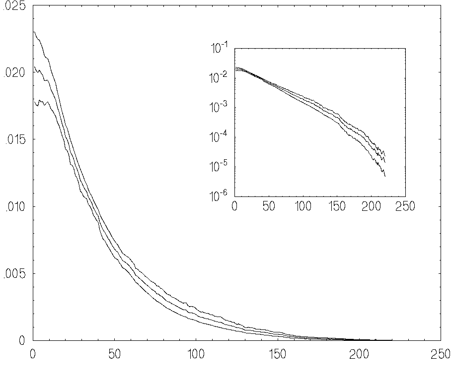
where n(t) is the solution of the integral equation Eq.(15) for the real histogram N(t), and n_j(t) is the solution of the integral equation for 'quasi-histogram' input data N_j(t). The muonium formation rate function n(t) in liquid helium at temperature T=0.7K is shown in Fig.3 together with the estimation of its statistical accuracy (at level $\pm1 \sigma$).

Fig.3. Muonium formation rate function n(t) in liquid He and its accuracy at the level $\pm \sigma$ (main plot). The same functions is shown in insert in logarithmic scale on Y axis. On X axis is the histogram bin numbers, one bin time $\Delta t=2.5$ ns. Temperature T=0.7K

It is seen from this figure that mean accuracy is less than 2% for total histogram statistics

$$\displaystyle \sum \limits_{i=1}^{4000} N(t_i) \sim 6 \cdot10^6 .$$

The function n(t) decreases to zero with increasing time faster than an exponential -- in another words the curve n(t) is upwards convex in Y logarithmic scale plot.